I’ve seen a few cases of people splitting AB tests with modulo arithmetic. This isn’t the best idea, something I’ll argue in this post. I’ll also put forward an alternative to modulo arithmetic splitting, which keeps a lot of its advantages, with few of its disadvantages.

Splitting with mods

A common solution to spitting AB tests is to use modulo arithmetic on a user ID. This is a common solution for several reasons:

• Very easy to implement. Especially when a test needs to be rolled out ASAP, and there’s no existing test infrastructure, it can be tempting to just slap a modulo arithemtic operator in there and call it a day.
• Memoryless: you don’t need to save how people were assigned, because it’s already recorded in their ID and the splitting method.

The problem with splitting with mods are:

• It scales very poorly. You need to be careful tests don’t overlap, which means that the numbers you use as the modulo need to be coprime. – And that in turn means no one should be using the same numbers, so you need a way to “reserve” a number for your use.
• Even when numbers are coprime, it’s still possible that the overlap will be large and that there will be too much overlap beween groups.

Solving the problem with hashes

A simple way to solve this is to find another, better way to transform IDs to groups. A way that I’ve used in the past goes like this:

1. Take the user ID (or the ID of whatever you’re splitting over)
2. And a salt, unique to the AB test (I use ticket numbers, because they tie things up nicely)
3. Concatenate them (with a comma or something in between)
4. Hash them with a hashing algorithm (I use MD5, because it is also present in many DB systems)
5. Take the first 6 characters of the hashed data, and convert it to an integer
6. Divide that integer by the largest 6 digit hex number (0xffffff). Be sure to use floating point division.
7. And then split people using that floating point number. You could also multiply 0xffffff by a proportion and test for less than or greater than.

As python code:

# First, all the imports for the whole example
from tqdm import tqdm_notebook
import hashlib
import pandas
import scipy.stats
from sklearn.metrics import mutual_info_score
import statsmodels.api as sm


def ab_split(id, salt, control_group_size):
    '''
    Returns 't' (for test) or 'c' (for control), based on the ID and salt.
    The control_group_size is a float, between 0 and 1, that sets how big the
    control group is.
    '''
    test_id = str(id) + '-' + str(salt)
    test_id_digest = hashlib.md5(test_id.encode('ascii')).hexdigest()
    test_id_first_digits = test_id_digest[:6]
    test_id_final_int = int(test_id_first_digits, 16)
    ab_split = (test_id_final_int/0xFFFFFF)
    
    if ab_split > control_group_size:
        return 't'
    else:
        return 'c'

As MySQL code:

-- Obviously, set ID, SALT and CONTROL_GROUP_SIZE as appropriate
SELECT if(
   conv(
      substr(
          md5(concat(ID, '-', SALT)),
          1, 6),
      16, 10)/0xffffff > CONTROL_GROUP_SIZE, 't', 'c')

Verifying the general solution

So, you need to ask: how random is this solution? There are a few ways to test it, but I think the neatest is to check three things:

1. Given some test data, how likely or unlikely is it that we see the observed number of treated cases. This checks whether we’re splitting correctly.
2. Given some test data, are we seeing random sequences of test and control, rather than have them all bunched up.
3. Given some test cases, how often does knowing about one AB test tell you something useful about another AB test.

Checking item 1

For this, I ran the test code over 10K IDs, and checked if the proportion of test users was plausible:

# Full example.
# First, generate the group

users = pandas.DataFrame({'id': np.arange(100**2)})
users['test_group'] = users.id.apply(lambda id: ab_split(id, 'ticket-1', 0.25))

dist = scipy.stats.binom(n=10000, p=0.25)
# Then, check that the number of users in the control group
# is a plausible size
print('Control group proportion ', (users.test_group == 'c').mean())
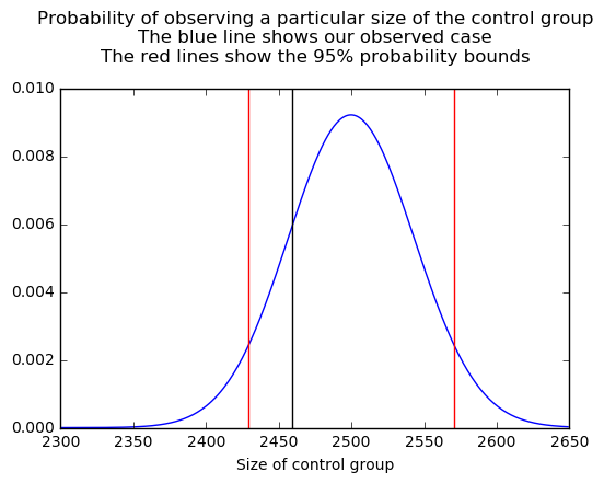
plot(np.arange(2300, 2650), dist.pmf(np.arange(2300, 2650)))
title('Probability of observing a particular size of the control group\n'
      'The blue line shows our observed case\n'
      'The red lines show the 95% probability bounds\n')
xlabel('Size of control group')

axvline((users.test_group == 'c').sum(), c='black')
axvline(dist.isf(0.95), c='red')
axvline(dist.isf(0.05), c='red')

We get a proportion of 0.2459, well inside the 95% CI for our expected distribution:

Checking item 2

The next thing to check is that the order of the ts and cs appears random. I’ve been learning about non-parametric statistics recently, and a lot of it is based around run tests. They test the randomness of a sequence, by looking at the length of runs of values. Compare these two sequences:

• tttttffff
• tttfftfft

While they both could be random, it seems like the second is “more random” than the first, and if you assume a random process produces the values, the run of five ts in the first is very unlikely, more unlikely than the run of length 3 in the second.

There’s a tool for testing this in the statsmodels package, stats.Runs, which returns the statistic and p-value as a tuple. We’re interested in the p-value.

print(sm.stats.Runs(np.random.choice(2, size=50)).runs_test()[1])
# Returns 0.559265850702 (no pattern)
print(sm.stats.Runs(np.concatenate([np.zeros(25), np.ones(25)])).runs_test()[1])
# Returns 6.9552625601e-12 (strong pattern)
print(sm.stats.Runs((users.test_group == 't').values.astype('int')).runs_test()[1])
# Returns 0.455721325515 (no pattern)

Checking item 3

The only thing left to check is the most important one: that a person’s group in one AB test has no effect on their group in another one.

For this, I’ve used mutual information, which measures the amount of information you get about a variable from another variable. For example, the mutual information between citizenship and country of residence is high, because generally people are citizens of where they live. In contrast, the mutual infomration between citizenship and whether someone just flipped a heads or tails on a coin is low, because they’re unrelated.

For this test, I used 200 different salts, and compared the mutual information between every combination of AB tests:

mat = np.zeros((200, 200))
# Hashing is much slower, so we need a cache to speed it up
series_cache = {}

for mod1 in tqdm_notebook(range(500, 700)):
    for mod2 in range(500, 700):
        if mod1 in series_cache:
            split1 = series_cache[mod1]
        else:
            split1 = users.id.apply(lambda id: ab_split(id, str(mod1), 0.5)) == 't'
            series_cache[mod1] = split1
            
        if mod2 in series_cache:
            split2 = series_cache[mod2]
        else:
            split2 = users.id.apply(lambda id: ab_split(id, str(mod2), 0.5)) == 't'
            series_cache[mod2] = split2
        mat[mod1-500, mod2-500] = mutual_info_score(split1, split2)
mat[np.diag_indices(200)] = np.NaN
matshow(log(0.001 + mat), cmap='viridis')
colorbar()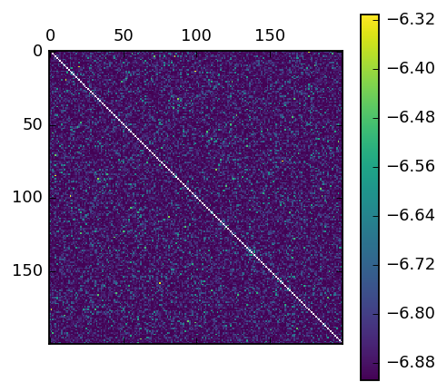

In contrast, here’s one for the naive modulo arithemetic approach:

mat = np.zeros((200, 200))
for mod1 in tqdm_notebook(range(2, 200)):
    for mod2 in range(2, 200):
        split1 = users.id % mod1 > mod1//2
        split2 = users.id % mod2 > mod2//2
        mat[mod1, mod2] = mutual_info_score(split1, split2)
mat[np.diag_indices(200)] = np.NaN
matshow(log(0.001 + mat), cmap='viridis')
colorbar()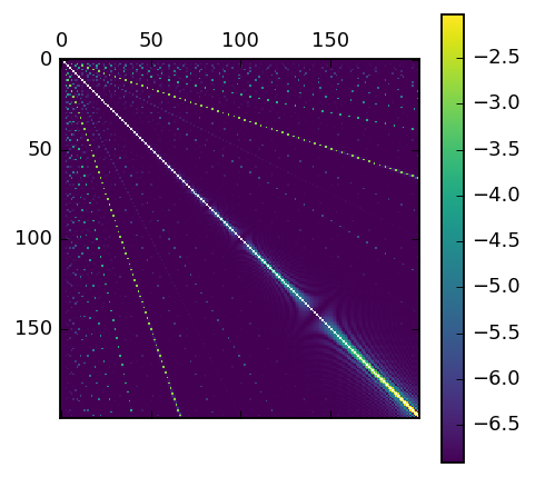

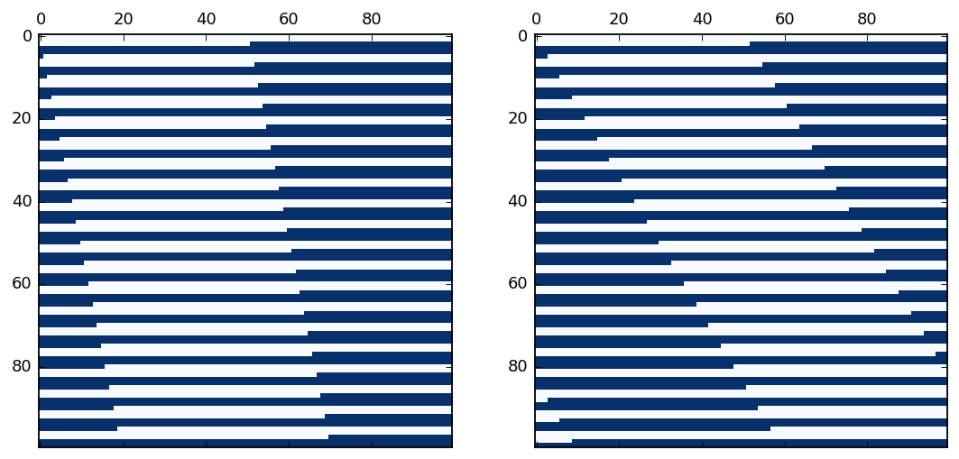
As you can see, there are heavy biases in it. You can also start to see another issue, on the diagonal in the bottom right, where large mods relative to the number of users mean there’s high overlap. Here’s three images that illustrate this effect. The first two are our 10K users (0-100 on the first line, 100-200 on the next and so on). They colored by test or control, using mods 501 and 503. As you can see, they look quite similar. Even those similarites would even out over a large number of users, for small number of users the splits are quite similar:

And this graph is the same as before, but mods up to 500-600, instead of 0-100, it becomes more obvious:

Things to look out for

When you implement this scheme, here are a few tips:

1. Watch out for numeric overflow. If you’re on a 32 bit system, and you use the first 8 digits of the MD5 sum, you may overflow into negative numbers, and throw everything off.
   • Be especially careful when you have multiple systems. The worst thing that can happen is that one system splits one way, and another splits in a different way, because of differences in the conversions on different platforms.
2. Even the smallest difference in the salts can totally ruin results. I suggest saving the first 10 or 20 IDs in the split (ie, run numbers 1 through 20 through the AB test function and save the results). This will be invaluable in working out which salt is correct if for some reason there is a proble.
3. Test for aggreement in libraries. Put 1 through 1000 through the AB test splitter, on every platform it is used on, and make sure they all agree. Use different salts as well.

Conclusion

This hashing approach is nice because it keeps a lot of the advantages of the modulo appraoch, with few of the disadvantages. I hope you find it useful!