For a while now, I’ve had a problem in PYMC3, where intercepts would “wander”. In this post, I explain,

How to fix this problem
An explanation of different ways to encode categorical values in linear models.

The notebook for this project can be found here.

Motivating example

I built a simple model, of the form y ~ C(a) + b + 1, and put it through pymc3. In the trace, you can see the “wandering” behaviour, which arises because pymc3 has a choice of where to put the constant value. It can either put the constant into the a values, or into the intercept, and either way is pretty much fine.

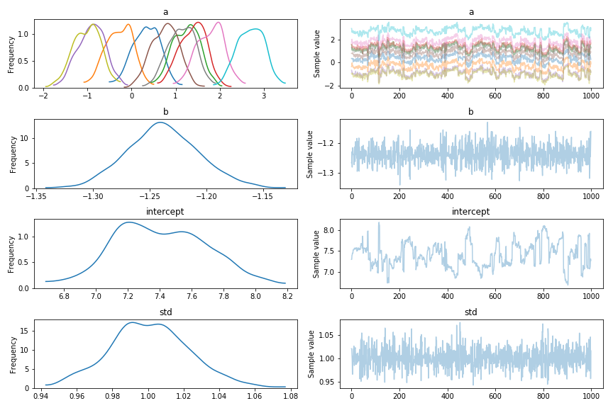
This leads to a number of problems: the model is very slow to run, I think because the NUTS sampler rejects many values before working out how it needs to share the wandering value. It also makes the results of the sampler very hard to use. As you can see, the different a values don’t settle down, meaning I can’t really infer things about them.

Dataset

The dataset is easy to build, simply:

np.random.seed(804188826)
n = 1000
a = np.random.choice(10, size=n)
a_value = np.random.normal(size=10)
b = np.random.normal(size=n)
b_coeff = np.random.normal(0, 5)
intercept = np.random.normal() + 10

y_underlying = a_value[a] + b*b_coeff + intercept
y = y_underlying + np.random.normal(size=n)

data_mat = pandas.DataFrame({
    'a': a,
    'b': b,
    'y': y,
})

Model

The model follows the basic structure of a lot of PYMC3 models. The problematic line is commented.

# Wandering example
with pm.Model() as model:
    a_coeff = pm.Normal('a', shape=10)
    b_coeff = pm.Normal('b')
    intercept = pm.Normal('intercept')
    sd = pm.HalfNormal('std')
    
    mu = (a_coeff[data_mat.a.values] +  # Right here was our mistake.
          data_mat.b.values * b_coeff +
          intercept)
    pm.Normal('obs', mu=mu, sd=sd, observed=data_mat.y.values)
    
    trace = pm.sample(1000)
    pm.traceplot(trace)
    ppc = pm.sample_ppc(trace)

Treatment coding

The problem here is that pymc3 even has a choice of where to put the constant term. In this model, it would be possible to remove the intercept term, but that wouldn’t really solve the problem when there are multiple constant terms. In order to solve this, it’s necessary to use better contrast encoding schemes. Contrast coding provides a better way to encode these constant parameters. The simplest way is “treatment” coding, which is basically one-hot encoding, but one of the options has no effect. Doing this enforces a constraint that the missing option has effect zero.

To do this, I recommend the patsy contrasts module.

cs = contrasts.Treatment().code_without_intercept(list(range(10)))

with pm.Model() as model:
    a_coeff = pm.Normal('a', shape=cs.matrix.shape[1])
    b_coeff = pm.Normal('b')
    intercept = pm.Normal('intercept')
    sd = pm.HalfNormal('std')
    
    mu = (theano.dot(cs.matrix[data_mat.a.values], a_coeff) +  # No longer a problem
          b_coeff * data_mat.b.values +
          intercept)
    pm.Normal('obs', mu=mu, sd=sd, observed=data_mat.y.values)
    
    trace = pm.sample(1000)
    pm.traceplot(trace)
    ppc = pm.sample_ppc(trace)

One other advantage of this is that the sampling is much faster in some cases.

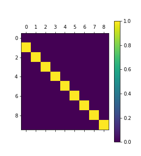
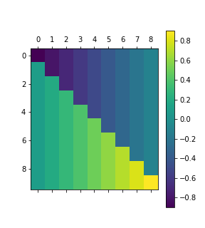
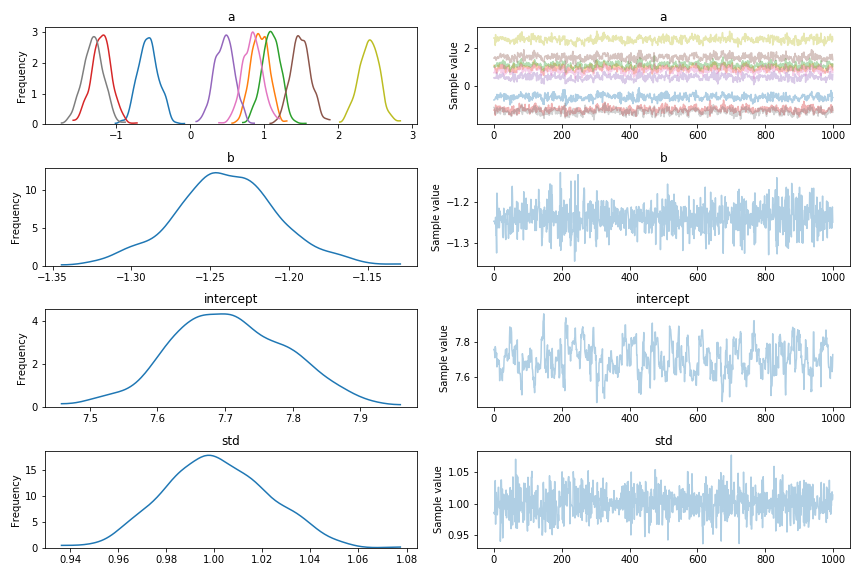You can see that the parameters no longer wander! Here’s the contents of the contrast matrix:

Sum coding

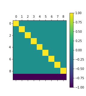
In treatment coding, one of the coefficients of a had zero effect, and all the others are expressed as deviations from that value. That’s neat, but another option might be to make all the treatments sum to zero:

cs = contrasts.Treatment().code_without_intercept(list(range(10)))

And proceeed as before. The coding has a final row of -1, rather than zero as before:

Diff coding

This is the last coding schema I’ll cover, it’s pretty weird. In diff coding, the coefficients are the differences between neighbouring coefficients:

 cs = contrasts.Diff().code_without_intercept(list(range(10)))

It’s contrast matrix looks interesting to say the least:

Different coding outputs

The best way to understand these differences is to look at the coefficients, and what we expect them to be.

To start with, here are all the different coefficients, side by side:

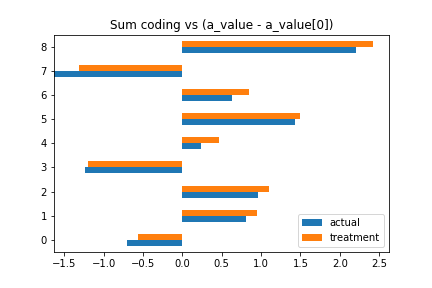
Treatment coding

In sum coding, the coefficients are the same as the original coefficients, minus the first coefficient:

pandas.DataFrame({
    'treatment': trace_trt['a'].mean(0),
    'actual': (a_value-a_value[0])[1:]
})

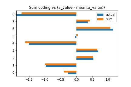
Sum coding

In sum coding, the coefficients are the same as the original coefficients, minus the mean of all coefficients, and ignoring the first coefficient.

pandas.DataFrame({
    'sum': trace_sum['a'].mean(0),
    'actual': (a_value-mean(a_value))[:-1]
})

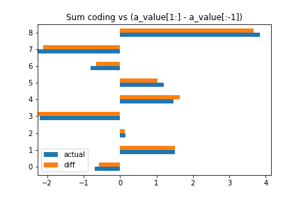
Diff coding

Diff coding is neat! Each coefficient is the difference with the coefficient preceding it! Now, I’m not sure why you’d need this, but you know, you do you.

pandas.DataFrame({
    'diff': trace_diff['a'].mean(0),
    'actual': a_value[1:] - a_value[:-1]
})

Conclusion & Discussion

One thing I now realize is that some of my decision heuristics have been broken for a long time. I’ve always assumed that having a positive coefficient in a category meant that that category had an effect. From these categorical codings, it’s clear that simply looking at each category isn’t enough. You need to look at all categories, together, and then link them back to the original question to properly answer it.

However, overall this approach solves the wandering problem, and adds in a bunch of new regression tricks for me to start considering.