Introduction

In this post, I’ll be describing how I implemented a zero-truncated poisson distribution in PyMC3, as well as why I did so.

What is truncation?

Truncated distributions arise when some parts of a distribution are impossible to observe. For example, consider how often someone visits a store in a week. It’s natural to count people from one, and it’s hard to imagine the people who didn’t visit. For example, do we assume that every single person in the world didn’t visit? All 7.6 billion of them?

It’s natural to use a Poisson distribution for counts like these, but unfortunately the poisson distribution can produce zero counts. Because there are no zero-counts, the poisson’s estimate of the average visiting rate is far higher than expected. This also causes something called overdispersion, where the estimated variance of the lambda value is higher than it needs to be, making it hard to compare different rates.

Example problem

See the accompanying notebook for the code.

In this problem, we’ll be working with a really simple dataset. In it, we have two groups of people, one with an average of 0.79 visits per week, the other with 0.95 visits per week:

lams = np.asarray([0.79, 0.95])                    # The two lambdas
choices = np.random.choice(2, size=4000)          # Pick 4000 people, and give them groups
full_counts = np.random.poisson(lams[choices])    # Count their visits
truncated_counts = full_counts[full_counts > 0]   # Remove any counts that are zero
truncated_choices = choices[full_counts > 0]      # And also find the groups for those non-zero visitors
trunc_size = truncated_counts.size 
colors = sns.color_palette(n_colors=2)

Non-truncated solution

Just to start off, we make sure that we an fit the non-truncated version:

with pm.Model():
    lam = pm.HalfNormal('lam', 10, shape=2)
    pm.Poisson('obs', 
        mu=lam[choices[:trunc_size]],      # We only take trunc_size values here,
        observed=full_counts[:trunc_size]) # because we want to make sure the tests are
                                           # given the same amount of data.
    trace = pm.sample(5000)
    ppc = pm.sample_ppc(trace)
    pm.traceplot(trace)
    
pm.summary(trace)

This works perfectly (that’s good), and here is the distribution of the two lambda values, as well as the true values (in blue and orange), and histograms for post-predictive checks:

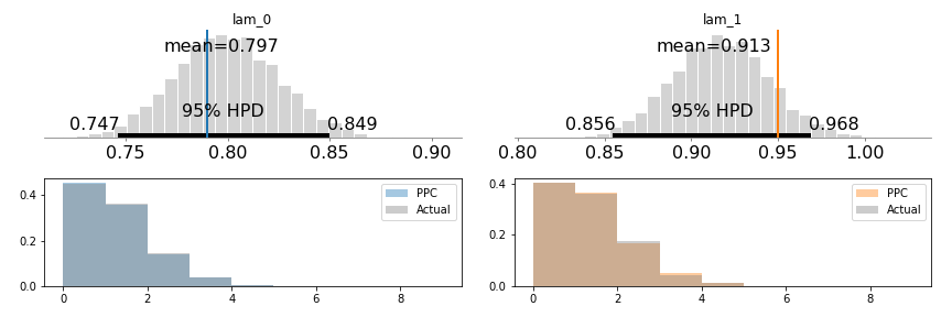
Generally, the 95% confidence intervals will not include each other (depending on the particulars of the random dataset). And also, the 95% CI contains the two lambda values we expect!

Naive solution

Here, we just use the poisson distribution and ignore any issues of truncation:

with pm.Model():
    lam = pm.HalfNormal('lam', 10, shape=2)
    pm.Poisson('obs', 
        mu=lam[choices[:trunc_size]], 
        observed=full_counts[:trunc_size])
    
    trace = pm.sample(5000)
    pm.traceplot(trace)

pm.summary(trace)

This distribution is less promising:

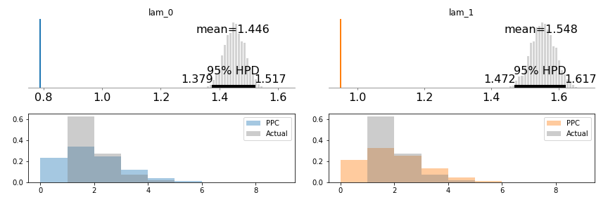
The lambdas recovered are far from where we’d expect them, and the HPD intervals sit over each other, suggesting that the two groups do not have different visit rates (even though we know they do). Lastly, the PPC checks are just way off - the two distributions are wildly different.

I also had some warnings while fitting this - PyMC3 is trying to tell me I messed up 😊.

Solution using a truncated distribution

I’ll go into the implementation of the zero-truncated poisson in the next section, but here’s an example of it in action;

with pm.Model():
    lam = pm.HalfNormal('lam', 10, shape=2)
    ZTP('obs', mu=lam[truncated_choices], observed=truncated_counts)
    
    trace = pm.sample(5000)
    pm.traceplot(trace)
pm.summary(trace)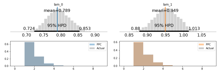

Notice here that we’ve successfully used the truncated data to retrieve the correct lambda values! Additionally, the two distribution’s HPD do not overlap, meaning that we’ve (correctly) inferred that there are different values for the two group’s visitation rates.

Things we’ve done:

With our zero-truncated poisson we’ve:

✔ Accounted for the truncated zero data
✔ correctly recovered underlying lambda values even when large parts of the dataset are unobserved
✔ managed to prove that there’s a significant difference between the two groups - impossible without accounting for the truncation.

Implementation

How’s it done? Two steps:

Use the truncated distribution formula to work out the log-pdf of the distribution.
Use the same formulas to work out the inverse-CDF of the new distribution
Implement the distribution in pymc3

Step 1

The poisson distribution’s PDF is \(\frac{\lambda^k e^{-\lambda}}{k!}\).

The new PDF is given by \(\frac{g(x)}{F(\infty) - F(0)}\) where \(F\) is the poisson CDF and \(g(x)\) is the modified PDF which is zero at \(x=0\).

What we’re doing here is cutting out part of the PDF (to make \(g(x)\)), and scaling the PDF to account for the missing probability. The poisson CDF is 1 at inifinity (remember that the CDF here represents the probability of seeing a count less than infinity - so its probability is one), so \(F(\infty) = 1\). \(F(0)\) is simply found by substituting it into the formula on wikipedia for the CDF of the poisson distribution. I used the summation approach - because it’s very simple:

\[e^{-\lambda}\sum_{i=0}^{0}\frac{\lambda^i}{i!}\]

Which of course simplifies to \(e^{-\lambda}\). The final formula is (click here for a derivation):

\[\frac{\lambda^k}{(e^\lambda-1)k!}\]

So now we simply take the log of this, and we get:

\[\log \lambda^k - \log(k!) - \log(e^\lambda - 1)\]

PyMC3 has a few useful functions here to help us out:

logpow: for taking the log of powers, with special cases for zeros
factln: a differential log-factorial

And the final expression is:

p = logpow(mu, value) - (factln(value) + pm.math.log(pm.math.exp(mu)-1))

Step 2

For this, we need a few ingredients:

a way to map random numbers in interval [0, 1) to the truncated interval
The ppf function, which is what scipy calls the inverse CDF

Then it’s simply a matter of taking the mapped numbers and then passing them through the ppf function of the existing poisson distribution.

I implemented this as a “scipy-like” function that I could pass in to PyMC3’s generate_samples method:

# This is part of the ZPT class
def zpt_cdf(self, lam, size=None):
    # get the lam value and produce the scipy frozen
    # poisson distribution using it
    lam = np.asarray(lam)
    dist = scipy.stats.distributions.poisson(lam)
    
    # find the lower CDF value, the probability of a 
    # zero (or lower) occuring. 
    lower_cdf = dist.cdf(0)
    # The upper CDF is 1, as we are not placing an upper
    # bound on this distribution
    upper_cdf = 1
    
    # Move our random sample into the truncated area of
    # the distribution
    shrink_factor = upper_cdf - lower_cdf
    sample = np.random.rand(size) * shrink_factor + lower_cdf
    
    # and find the value of the poisson distribution
    # at those sampled points. In this case, this will
    # mean no zeros.
    return dist.ppf(sample)

Step 3

import pymc3 as pm
from pymc3.distributions.dist_math import bound, logpow, factln
from pymc3.distributions import draw_values, generate_samples
import theano.tensor as tt
import numpy as np
import scipy.stats.distributions

class ZTP(pm.Discrete):
    def __init__(self, mu, *args, **kwargs):
        super().__init__(*args, **kwargs)
        # The mode of the poisson is given by floor(mu), but if this is 
        # zero we use 1 instead as it's the next most-frequent value.
        self.mode = tt.maximum(tt.floor(mu).astype('int32'), 1)
        self.mu = mu = tt.as_tensor_variable(mu)

    def zpt_cdf(self, mu, size=None):
        mu = np.asarray(mu)
        dist = scipy.stats.distributions.poisson(mu)
        
        lower_cdf = dist.cdf(0)
        upper_cdf = 1
        nrm = upper_cdf - lower_cdf
        sample = np.random.rand(size) * nrm + lower_cdf

        return dist.ppf(sample)
        
    def random(self, point=None, size=None, repeat=None):
        mu = draw_values([self.mu], point=point)
        return generate_samples(self.zpt_cdf, mu,
                                dist_shape=self.shape,
                                size=size)

    def logp(self, value):
        mu = self.mu
        log_prob = bound(
            p,
            mu >= 0, value >= 0)
        # Return zero when mu and value are both zero
        return tt.switch(1 * tt.eq(mu, 0) * tt.eq(value, 0),
                         0, log_prob)

Conclusion

Hopefully at this point you’ve seen the importance of accoutning for truncated data - if you want to the the right results, you should be checking for truncation effects. And hopefully I’ve given you enough of a starting point to write your own truncated distributions, should the need arise.

Happy sampling!